R Deep Learning Cookbook Pdf Download

Deep learning has transformed many traditional businesses, such as web search, advertising, and many more. A major challenge with the traditional machine learning approaches isthat we need to spend a considerable amount of time choosing the most appropriate feature selection process before modeling. Besides this, these traditional techniques operate with some level of human intervention and guidance. However, with deep learning algorithms, we can get rid of the overhead of explicit feature selection since it is taken care of by the models themselves.These deep learning algorithms are capable of modeling complex and non-linear relationships within the data.In this book, we'll introduce you to how to set up a deep learning ecosystem in R.Deep neural networks use sophisticated mathematical modeling techniques to process data in complex ways. In this book, we'llshowcase the use of various deep learning libraries, such askeras and MXNet, so that you can utilize their enriched set of functions and capabilities in order to build and execute deep learning models, although we'll primarily focus on working with thekeras library. These libraries come withCPU and GPU support and are user-friendly so that you can prototype deep learning models quickly.

In this chapter, we will demonstrate how to set up a deep learning environment in R. You will also get familiar with various TensorFlow APIs and how to implement a neural network using them. You will also learn how to tune the various parameters of a neural network and also gain an understanding of various activation functions and their usage for different types of problem statements.

In this chapter, we will cover the following recipes:

• Setting up the environment
• Implementing neural networks with Keras
• TensorFlow Estimator API
• TensorFlow Core API
• Implementing a single-layer neural network
• Training your first deep neural network

Before implementing a deep neural network, we need to set up our system and configure it so that we can apply a variety of deep learning techniques. This recipe assumes that you have the Anaconda distribution installed on your system.

Let's configure our system for deep learning. It is recommended that you create a deep learning environment in Anaconda. If you have an older version of R in the conda environment, you need to update your R version to 3.5.x or above.

You also need to install the CUDA and cuDNN libraries for GPU support. You can read more about the prerequisites at https://tensorflow.rstudio.com/tools/local_gpu.html#prerequisties.

Please note that if your system does not have NVIDIA graphics support, then GPU processing cannot be done.

Let's create an environment in Anaconda (ensure that you have R and Python installed):

1. Go to Anaconda Navigator from the Start menu.
2. Click on Environments.
3. Create a new environment and name it. Make sure that both the Python and R options are selected, as shown in the following screenshot:

4. Install the keras library in R using the following command in RStudio or by using theTerminal of the conda environment created in the previous step:

install.packages("keras")

5. Install keras with the tensorflow backend.

The keras library supports TensorFlow as the default backend. Theano and CNTK are other alternative backends that can be used instead of TensorFlow.

To install the CPU version, please refer to the following code:

                  install_keras                  (                  method                                                      =                                                      c                  (                  "auto"                  ,                                    "virtualenv"                  ,                                    "conda"                  ),                                                      conda                                                      =                                                      "auto"                  ,                                    version                                                      =                                                      "default"                  ,                                    tensorflow                                                      =                                                      "default"                  ,                                                      extra_packages                                                      =                                                      c                  (                  "tensorflow-hub"                  ))                

To install the GPU version, please refer to the following steps:

1. Ensure that you have met all the installation prerequisites, including installing the CUDA and cuDNN libraries.
2. Set thetensorflow argument's value togpu  in the install_keras() function:

install_keras(tensorflow = "gpu")

The preceding command will install the GPU version of keras in R.

Keras and TensorFlow programs can be executed on both CPUs and GPUs, though these programs usually run faster on GPUs.If your system does not support an NVIDIA GPU, you only need to install the CPU version. However , if your system has an NVIDIA GPU that meets all the prerequisites and you need to run performance-critical applications, you should install the GPU version. To run the GPU version of TensorFlow, we need an NVIDIA GPU, and then we need to install a variety of software components (CUDA Toolkit v9.0, NVIDIA drivers, and cuDNN v7.0) on the system.

In steps 1 to 3, we created a new conda environment with both the R and Python kernels installed. In steps 4 and 5, we installed the keras library in the environment we created.

The only supported installation method on Windows is conda. Therefore, you should install Anaconda 3.x for Windows before installing keras. The keras package uses the TensorFlow backend by default. If you want to switch to Theano or CNTK, call the use_backend() function after loading the keras library.

For the Theano backend, use the following command:

library(keras)
use_backend("theano")

For the CNTK backend,use the following command:

library(keras)
use_backend("cntk")

Now, your system is ready to train deep learning models.

You can find out more about the GPU version installation of keras and its prerequisites here: https://tensorflow.rstudio.com/tools/local_gpu.html.

TensorFlow is an open source software library developed by Google for numerical computation using data flow graphs. The R interface for TensorFlow is developed by RStudio, which provides an interface for three TensorFlow APIs:

• Keras
• Estimator
• Core

The keras, tfestimators, and tensorflow packages provide R interfaces to the aforementioned APIs, respectively. Keras and Estimator are high-level APIs, while Core is a low-level API that offers full access to the core of TensorFlow. In this recipe, we will demonstrate how we can build and train deep learning models using Keras.

Keras is a high-level neural network API, written in Python and capable of running on top of TensorFlow, CNTK, or Theano. The R interface for Keras uses TensorFlow as its default backend engine. Thekeras package provides an R interface for the TensorFlow Keras API. It lets you build deep learning models in two ways, sequential and functional, both of which will be described in the following sections.

Keras's Sequential API is straightforward to understand and implement. It lets us create a neural network linearly; that is, we can build a neural network layer-by-layer where we initialize a sequential model and then stack a series of hidden and output layers on it.

Before creating a neural network using the Sequential API, let's load the keras library into our environment and generate some dummy data:

library(keras)

Now, let's simulate some dummy data for this exercise:

x_data <- matrix(rnorm(1000*784), nrow = 1000, ncol = 784)
y_data <- matrix(rnorm(1000), nrow = 1000, ncol = 1)

We can check the dimension of the x and y data by executing the following commands:

dim(x_data)
dim(y_data)

The dimension of the x_data data is 1,000×784, whereas the dimension of the y_data data is 1,000×1.

Now, we can build our first sequential keras model and train it:

1. Let's start by defining a sequential model:

model_sequential <- keras_model_sequential()

2. We need to add layers to the model we defined in the preceding code block:

model_sequential %>%                  
layer_dense(units = 16,batch_size = ,input_shape = c(784)) %>%                  
layer_activation('relu') %>%                  
layer_dense(units = 1)

3. After adding the layers to our model, we need to compile it:

model_sequential %>% compile(
                  loss = "mse",
                  optimizer = optimizer_sgd(),
                  metrics = list("mean_absolute_error")
)

4. Now, let's visualize the summary of the model we created:

model_sequential %>% summary()

The summary of the model is as follows:

5. Now, let's train the model and store the training stats in a variable in order to plot the model's metrics:

history <- model_sequential %>% fit(
                  x_data,                  
                  y_data,
                  epochs = 30,
                  batch_size = 128,                  
                  validation_split = 0.2
)
# Plotting model metrics
plot(history)
                

The preceding code generates the following plot:

The preceding plot shows the loss and mean absolute error for the training and validation data.

In step 1, we initialized a sequential model by calling thekeras_model_sequential() function. In the next step, we stacked hidden and output layers by using a series of layer functions. The layer_dense() function adds a densely-connected layer to the defined model. The first layer of the sequential model needs to know what input shape it should expect, so we passed a value to theinput_shape argument of the first layer. In our case, the input shape was equal to the number of features in the dataset. When we add layers to the keras sequential model, the model object is modified in-place, and we do not need to assign the updated object back to the original. The keras object's behavior is unlike most R objects (R objects are typically immutable). For our model, we used therelu activation function. Thelayer_activation() function creates an activation layer that takes input from the preceding hidden layer and applies activation to the output of our previous hidden layer. We can also use different functions, such as leaky ReLU, softmax, and more (activation functions will be discussed in Implementing a single-layer neural network recipe). In the output layer of our model, no activation was applied.

We can also implement various activation functions for each layer by passing a value to theactivation argument in the layer_dense() function instead of adding an activation layer explicitly. It applies the following operation:

output=activation(dot(input, kernel)+bias)

Here, the activation argument refers to the element-wise activation function that's passed, while thekernel is a weights matrix that's created by the layer. The bias is a bias vector that's produced by the layer.

To train a model, we need to configure the learning process. We did this instep 3 using the compile() function. In our training process, we applied a stochastic gradient descent optimizer to find the weights and biases that minimize our objective loss function; that is, the mean squared error. Themetrics argument calculates the metric to be evaluated by the model during training and testing.

In step 4, we looked at the summary of the model; it showed us information about each layer, such as the shape of the output of each layer and the parameters of each layer.

In the last step, we trained our model for a fixed number of iterations on the dataset. Here, theepochs argument defines the number of iterations. Thevalidation_split argument can take float values between 0 and 1. It specifies a fraction of the training data to be used as validation data. Finally,batch_size defines the number of samples that propagate through the network.

Training a deep learning model is a time-consuming task. If training stops unexpectedly, we can lose a lot of our work. The keras library in R provides us with the functionality to save a model's progress during and after training. A saved model contains the weight values, the model's configuration, and the optimizer's configuration. If the training process is interrupted somehow, we can pick up training from there.

The following code block shows how we can save the model after training:

# Save model
model_sequential %>% save_model_hdf5("my_model.h5")

If we want to save the model after each iteration while training, we need to create a checkpoint object. To perform this task, we use thecallback_model_checkpoint() function. The value of the filepath argument defines the name of the model that we want to save at the end of each iteration. For example, if filepath is {epoch:02d}-{val_loss:.2f}.hdf5, the model will be saved with the epoch number and the validation loss in the filename.

The following code block demonstrates how to save a model after each epoch:

checkpoint_dir <- "checkpoints"
dir.create(checkpoint_dir, showWarnings = FALSE)
filepath <- file.path(checkpoint_dir, "{epoch:02d}.hdf5")
# Create checkpoint callback
cp_callback <- callback_model_checkpoint(
                    filepath = filepath,
                    verbose = 1
)
                  
# Fit model and save model after each check point                    
model_sequential %>% fit(
                    x_data,                    
                    y_data,
                    epochs = 30,
                    batch_size = 128,                    
                    validation_split = 0.2,
                    callbacks = list(cp_callback)
)
                

By doing this, you've learned how to save models with the appropriate checkpoints and callbacks.

• To find out more about writing custom layers in Keras, go to https://tensorflow.rstudio.com/keras/articles/custom_layers.html.

Keras's functional API gives us more flexibility when it comes to building complex models. We can create non-sequential connections between layers, multiple inputs/outputs models, or models with shared layers or models that reuse layers.

In this section, we will use the same simulated dataset that we created in the previous section of this recipe, Sequential API. Here, we will create a multi-output functional model:

1. Let's start by importing the required library and create an input layer:

library(keras)
# input layer
inputs <- layer_input(shape = c(784))
                

2. Next, we need to define two outputs:

predictions1 <- inputs %>%
                  layer_dense(units = 8)%>%
                  layer_activation('relu') %>%
                  layer_dense(units = 1,name = "pred_1")
predictions2 <- inputs %>%
                    layer_dense(units = 16)%>%
                    layer_activation('tanh') %>%
                    layer_dense(units = 1,name = "pred_2")
                

3. Now, we need to define a functional Keras model:

model_functional = keras_model(inputs = inputs,outputs = c(predictions1,predictions2))

Let's look at the summary of the model:

summary(model_functional)

The following screenshot shows the model's summary:

4. Now, we compile our model:

model_functional %>% compile(
                  loss = "mse",
                  optimizer = optimizer_rmsprop(),
                  metrics = list("mean_absolute_error")
)

5. Next, we need to train the model and visualize the model's parameters:

history_functional <- model_functional %>% fit(
                  x_data,
                  list(y_data,y_data),
                  epochs = 30,
                  batch_size = 128,
                  validation_split = 0.2
                  )

Now, let's plot the model loss for the training and validation data of prediction 1 and prediction 2:

# Plot the model loss of the prediction 1 training data
plot(history_functional$metrics$pred_1_loss, main="Model Loss", xlab = "epoch", ylab="loss", col="blue", type="l")
# Plot the model loss of the prediction 1 validation data
lines(history_functional$metrics$val_pred_1_loss, col="green")
                  
# Plot the model loss of the prediction 2 training data
lines(history_functional$metrics$pred_2_loss, col="red")
                  
# Plot the model loss of the prediction 2 validation data
lines(history_functional$metrics$val_pred_2_loss, col="black")
                  
# Add legend
legend("topright", c("training loss prediction 1","validation loss prediction 1","training loss prediction 2","validation loss prediction 2"), col=c("blue", "green","red","black"), lty=c(1,1))
                

The following plot shows the training and validation loss for both prediction 1 and prediction 2:

Now, let's plot the mean absolute error for the training and validation data of prediction 1 and prediction 2:

# Plot the model mean absolute error of the prediction 1 training data
plot(history_functional$metrics$pred_1_mean_absolute_error, main="Mean Absolute Error", xlab = "epoch", ylab="error", col="blue", type="l")
# Plot the model mean squared error of the prediction 1 validation data
lines(history_functional$metrics$val_pred_1_mean_absolute_error, col="green")
                  
# Plot the model mean squared error of the prediction 2 training data
lines(history_functional$metrics$pred_2_mean_absolute_error, col="red")
                  
# Plot the model mean squared error of the prediction 2 validation data
lines(history_functional$metrics$val_pred_2_mean_absolute_error, col="black")
                  
# Add legend
legend("topright", c("training mean absolute error prediction 1","validation mean absolute error prediction 1","training mean absolute error prediction 2","validation mean absolute error prediction 2"), col=c("blue", "green","red","black"), lty=c(1,1))
                

The following plot shows the mean absolute errors for prediction 1 and prediction 2:

To create a model using the functional API, we need to create the input and output layers independently, and then pass them to thekeras_model() function in order to define the complete model. In the previous section, we created a model with two different output layers that share an input layer/tensor.

In step 1 , we created an input tensor using thelayer_input() function, which is an entry point into a computation graph that's been generated by the keras model. In step 2 , we defined two different output layers. These output layers have different configurations; that is, activation functions and the number of perceptron units. The input tensor flows through these and produces two different outputs.

In step 3, we defined our model using thekeras_model() function. It takes two arguments:inputsand outputs. These arguments specify which layers act as the input and output layers of the model. In the case of multi-input or multi-output models, you can use a vector of input layers and output layers, as shown here:

keras_model(inputs= c(input_layer_1, input_layer_2), outputs= c(output_layer_1, output_layer_2))

After we configured our model, we defined the learning process, trained our model, and visualized the loss and accuracy metrics. Thecompile() and fit() functions, which we used in steps 4 and 5, were described in detail in the How it works  sectionof the Sequential API  recipe.

You will come across scenarios where you'll want the output of one model in order to feed it into another model alongside another input. Thelayer_concatenate() function can be used to do this. Let's define a new input that we will concatenate with the predictions1 output layer wedefined in theHow to do it section of this recipe and build a model:

# Define new input of the model                  
new_input <- layer_input(shape = c(5), name = "new_input")
# Define output layer of new model
main_output <- layer_concatenate(c(predictions1, new_input)) %>%                    
                    layer_dense(units = 64, activation = 'relu') %>%
                    layer_dense(units = 1, activation = 'sigmoid', name = 'main_output')
                  
# We define a multi input and multi output model
model <- keras_model(
                    inputs = c(inputs, new_input),                    
                    outputs = c(predictions1, main_output)
)
                

 We can visualize the summary of the model using the summary() function.

It is good practice to give different layers unique names while working with complex models.

The Estimator is a high-level TensorFlow API that makes developing deep learning models much more manageable since you can use them to write models with high-level intuitive code. It builds a computation graph and provides an environment where we can initialize variables, load data, handle exceptions, and create checkpoints.

The tfestimators package is an R interface for the TensorFlow Estimator API. It implements various components of the TensorFlow Estimator API in R, as well as many pre-built canned models, such as linear models and deep neural networks (DNN classifiers and regressors). These are called pre-made estimators. The Estimator API does not have a direct implementation of recurrent neural networks or convolutional neural networks but supports a flexible framework for defining arbitrary new model types. This is known as the custom estimators framework.

In this recipe, we'll demonstrate how to build and fit a deep learning model using the Estimator API. To use the Estimator API in R, we need to install the tfestimators package.

First, let's install the library and then import it into our environment:

install.packages("tfestimators")
library(tfestimators)

Next, we need to simulate some dummy data for this exercise:

x_data_df <- as.data.frame( matrix(rnorm(1000*784), nrow = 1000, ncol = 784))
y_data_df <- as.data.frame(matrix(rnorm(1000), nrow = 1000, ncol = 1))

Let's rename the response variable totarget:

colnames(y_data_df)<- c("target")

Now, let's bind the x and y data together to prepare the training data:

dummy_data_estimator <- cbind(x_data_df,y_data_df)

By doing this, we have created our input dataset.

In this recipe, we will use a pre-made dnn_regressor estimator. Let's get started and build and train a deep learning estimator model:

1. We need to execute some steps before building an estimator neural network. First, we need to create a vector of feature names:

features_set <- setdiff(names(dummy_data_estimator), "target")

Here, we construct the feature columns according to the Estimator API. Thefeature_columns() function is a constructor for feature columns, which defines the expected shape of the input to the model:

feature_cols <- feature_columns(
                  column_numeric(features_set)
)

2. Next, we define an input function so that we canselect feature and response variables:

estimator_input_fn <- function(data_,num_epochs = 1) {
                  input_fn(data_, features = features_set, response = "target",num_epochs = num_epochs )
}

3. Let's construct an estimator regressor model:

regressor <- dnn_regressor(
                  feature_columns = feature_cols,
                  hidden_units = c(5, 10, 8),
                  label_dimension = 1L,
                  activation_fn = "relu"
)

4. Next, we need to train the regressor we built in the previous step:

train(regressor, input_fn = estimator_input_fn(data_ = dummy_data_estimator))

5. Similar to what we did for the training data, we need to simulate some test data and evaluate the model's performance:

x_data_test_df <- as.data.frame( matrix(rnorm(100*784), nrow = 100, ncol = 784))
y_data_test_df <- as.data.frame(matrix(rnorm(100), nrow = 100, ncol = 1))

We need to change the column name of the response variable, just like we did for the training data:

colnames(y_data_test_df)<- c("target")

We bind the x and y data together for the test data:

dummy_data_test_df <- cbind(x_data_test_df,y_data_test_df)

Now, we generate predictions for the test dataset using the regressor model we built previously:

predictions <- predict(regressor, input_fn = estimator_input_fn(dummy_data_test_df), predict_keys = c("predictions"))

Next, we evaluate the model's performance on the test dataset:

evaluation <- evaluate(regressor, input_fn = estimator_input_fn(dummy_data_test_df))
evaluation

In the next section, you will gain a comprehensive understanding of the steps we implemented here.

In this recipe, we implemented a DNN regressor using a pre-made estimator; the preceding program can be divided into a variety of subparts, as follows:

• Define the feature columns : In step 1, we created a vector of strings, which contains the names of our numeric feature columns. Next, we called thefeature_columns() function, which defines the expected shape value of an input tensor and how features should be transformed (numeric or categorical) while they're being modeled. In our case, the shape of the input tensor was 784, and all the values of the input tensor were numerical. We transform the numeric features by providing the names of the numeric columns to thecolumn_numeric() function within feature_columns(). If you have categorical columns in your data that have values such ascategory_x, category_y and you want to assign integer values (0, 1) to these, you can do this using thecolumn_categorical_with_identity() function.
• Write the dataset import functions : In step 2, we defined how a pre-made estimator receives data. It is defined by theinput_fn() function. It converts raw data sources into tensors and selects feature and response columns. It also configures how data is drawn during training; that is, shuffling, batch size, epochs, and so on.
• Instantiate the relevant pre-made Estimator : In step 3, we instantiated a pre-made deep neural network (DNN) estimator by calling dnn_regressor(). The hidden_units argument value of the function defines our network; that is, the hidden layers in the network and the number of perceptrons in each layer. It consists of dense, feedforward neural network layers. It takes vectors of integers as the argument value. In our model, we had three layers with 5, 10, and 8 perceptrons, respectively. We used relu as our activation function. The label_dimension argument of the dnn_regrssor function defines the shape of the regression target per example.
• Call a training, evaluation method : In step 4, we trained our model, and in the next step, we predicted the values for the test dataset and evaluated the performance of the model.

Estimators provide a utility called run hooks so that we can track training, report progress, request early stopping, and more. One such utility is the hook_history_saver() function, which lets us save training history in every training step. While training an estimator, we pass our run hooks' definition to the hooks argument of the train() function, as shown in the following code block. It saves model progress after every two training iterations and returns saved training metrics.

The following code block shows how to implement run hooks:

training_history <- train(regressor,
                  input_fn = estimator_input_fn(data_ = dummy_data_estimator),
                  hooks = list(hook_history_saver(every_n_step = 2))
                  )

Other pre-built run hooks are provided by the Estimator API. To find out more about them, please refer to the links in theSee also section of this recipe.

• Custom estimators: https://tensorflow.rstudio.com/tfestimators/articles/creating_estimators.html
• Otherpre-built run hooks: https://tensorflow.rstudio.com/tfestimators/articles/run_hooks.html
• Dataset API: https://tensorflow.rstudio.com/tfestimators/articles/dataset_api.html

The TensorFlow Core API is a set of modules written in Python. It is a system where computations are represented as graphs. The R tensorflow package provides complete access to the TensorFlow API from R. TensorFlow represents computations as a data flow graph, where each node represents a mathematical operation, and directed arcs represent a multidimensional data array or tensor that operations are performed on. In this recipe, we'll build and train a model using the R interface for the TensorFlow Core API.

You will need the tensorflow library installed to continue with this recipe. You can install it using the following command:

install.packages("tensorflow")

After installing the package, load it into your environment:

library(tensorflow)

Executing the two preceding code blocks doesn't install tensorflow completely. Here, we need to use the install_tensorflow() function to install TensorFlow, as shown in the following code block:

install_tensorflow()

TensorFlow installation in R needs a Python environment with the tensorflow library installed in it. The install_tensorflow() function attempts to create an isolated python environment calledr-tensorflow by default and installs tensorflow in it. It takes different values for the method argument,which provides various installation behaviors. These methods are explained at the following link: https://tensorflow.rstudio.com/tensorflow/articles/installation.html#installation-methods.

The virtualenv and conda methods are available on Linux and OS X, while the conda and system methods are available on Windows.

After the initial installation and setup, we can start building deep learning models by simply loading the TensorFlow library into the R environment:

1. Let's start by simulating some dummy data:

x_data = matrix(runif(1000*2),nrow = 1000,ncol = 1)
y_data = matrix(runif(1000),nrow = 1000,ncol = 1)

2. Now, we need to initialize some TensorFlow variables; that is, the weights and biases:

W <- tf$Variable(tf$random_uniform(shape(1L), -1.0, 1.0))
b <- tf$Variable(tf$zeros(shape(1L)))

3. Now, let's define the model:

y_hat <- W * x_data + b

4. Then, we need to define the loss function and optimizer:

loss <- tf$reduce_mean((y_hat - y_data) ^ 2)
optimizer <- tf$train$GradientDescentOptimizer(0.5)
train <- optimizer$minimize(loss)

5. Next, we launch the computation graph and initialize the TensorFlowvariables:

sess = tf$Session()
sess$run(tf$global_variables_initializer())

6. We train the model to fit the training data:

for (step in 1:201) {
                  sess$run(train)
                  if (step %% 20 == 0)
                  cat(step, "-", sess$run(W), sess$run(b), "\n")
}

Finally, we close the session:

sess$close()

Here are the results of every 20th iteration:

It is important that we close the session because resources are not released until we close it.

TensorFlow programs generate a computation graph in which the nodes of the graph are called ops. These ops take tensors as input and perform computations and produce tensors (tensors are n-dimensional arrays or lists). TensorFlow programs are structured in two phases: the construction phase and the execution phase. In the construction phase, we assemble the graph, while in the execution phase, we execute the graphs in the context of the session. Calling the tensorflow package in R creates an entry point (thetf object) to the TensorFlow API,through which we can access the main TensorFlow module. Thetf$Variable() function creates a variable that holds and updates trainable parameters. TensorFlow variables are in-memory buffers containing tensors.

In step 1, we created some dummy data. In the next step, we created two tf variables for the weights and bias with initial values.In step 3, we defined the model. In step 4, we defined the loss function, as per the following equation:

The reduce_mean() function computes the mean of the elements across the dimensions of a tensor. In our code, it calculates the average loss over the training set. In this step, we also defined the optimization algorithm we need to use to train our network. Here, we used the gradient descent optimizer with a learning rate of 0.5. Then, we defined the objective of each training step; that is, we minimize loss.

In step 5, we assembled the computation graph and provided TensorFlow with a description of the computations that we wanted to execute. In our implementation, we wanted TensorFlow to minimize loss; that is, minimize the mean squared error using the gradient descent algorithm. TensorFlow does not run any computations until the session is created and therun() function is called. We launched the session and added an ops (node) in order to run  sometf variable initializers. sess r u n ( t f run(tf global_variables_initializer()) initializes all the variables simultaneously. We should only run this ops after we have fully constructed the graph and launched it in a session. Finally, in the last step, we executed the training steps in a loop and printed the tf variables (the weight and bias) at each iteration.

It is suggested that you use one of the higher-level APIs (Keras or Estimator) rather than the lower-level core TensorFlow API.

An artificial neural network is a network of computing entities that can perform various tasks, such as regression, classification, clustering, and feature extraction. They are inspired by biological neural networks in the human brain. The most fundamental unit of a neural network is called a neuron/perceptron. A neuron is a simple computing unit that takes in a set of inputs and applies a function to these inputs in order to produce output.

The following diagram shows a simple neuron:

In 1957, Frank Rosenblatt proposed a classical perceptron model in which he associated weight with each input. He also proposed a method to realize these weights. A perceptron model is a simple computing unit with a threshold,, which can be defined by the following equation:

The following diagram represents a perceptron:

Perceptrons can only deal with linearly separable cases. The neural networks that we use today make use of activation functions rather than a harsh threshold, which are used in perceptrons. Unlike perceptrons, neural networks with non-linear activation functions can learn complex non-linear functional mappings between inputs and outputs, making them favorable for more complicated applications such as image recognition, language translation, speech recognition, and so on. The most popular activation functions are sigmoid, tanh, relu, and softmax.

We can implement various machine learning algorithms, such as simple linear regression, logistic regression, and so on, using neural networks. For example, we can think of logistic regression as a single-layer neural network. A logistic regression neural network uses a sigmoid () activation function. The following diagram shows a logistic regression neural network:

The output of the network is given as follows:

where z is equal to

While implementing a multinomial logistic regression problem using neural networks, we place a softmax activation function in the output layer. The following equation shows the output of a multinomial logistic regression neural network:

where z is the weighted sum of inputs for the j^th class

In neural networks, the network error is calculated by comparing the model's output to the desired output. This error term is used to guide the training of neural networks. After each training iteration, the error is communicated backward in the network and the weights of the network are updated in order to minimize the error. This process is called backpropagation. In this recipe, we will build a multi-class classification neural network using thekeras library in R.

We will use theiris dataset in this recipe. It is a multivariate dataset that consists of 50 samples that belong to three species of iris flower— setosa, virginica, and versicolor. Each sample contains four feature measurements; that is, the length and width of the sepals and petals in centimeters. We will use the keras package in order to utilize the deep learning functions for classification and the datasets library to import the iris dataset:

library(keras)
library(datasets)

In the next section, we will look at the data in more detail.

Before doing any transformations in the dataset, we will analyze the properties of the data, such as its dimensions, its variables, and its summary:

1. Let's start  by loading the iris dataset from thedatasets library:

data <- datasets::iris

Now, we can view the dimensions of the data:

dim(data)

Here, we can see that there are 150 rows and 5 columns in the data:

Let's display the first five records of the data:

head(data)

Let's have a glance at the data:

Now, let's have a look at the datatypes of the variables in the dataset:

str(data)

Here, we can see that all the columns except Species are numeric. Species is the response variable for this classification exercise:

Let's also look at a summary of the data to see the distribution of the variables:

summary(data)

We get the following output:

2. Now, we can work on the data transformation. To work with thekeras package, we need to convert the data into an array or a matrix. The matrix data elements should be of the same basic type, but here, we have target values that are of the factor type, so we need to change this:

# Converting the data into a matrix for keras to consume
data[,5] <- as.numeric(data[,5]) -1
data <- as.matrix(data)
# Setting dimnames of data to NULL
dimnames(data) <- NULL                      
                    head(data)
                

3. Now, we need to split the data into training and testing datasets. The seed number is the starting point that's used when generating a sequence of random numbers. Using the same number inside the function ensures that we can reproduce the same data each time the code is run:

set.seed(76)
# Training and testing data sample size
indexes <- sample(2,nrow(data),replace = TRUE,prob = c(0.70,0.30))
                

We divide the data in the ratio of 70:30 for the training and testing datasets, respectively:

# Splitting the predictor variables into training and testing
data.train <- data[indexes==1, 1:4]
data.test <- data[indexes==2, 1:4]
# Splitting the label attribute(response variable)into training and testing
data.trainingtarget <- data[indexes==1, 5]
data.testtarget <- data[indexes==2, 5]
                

4. Next, we one-hot encode the target column of the training and test data. Theto_categorical() function converts a class vector into a binary class matrix:

data.trainLabels <- to_categorical(data.trainingtarget)
data.testLabels <- to_categorical(data.testtarget)

5. Now, let's build the model and compile it. First, we need to initialize a Keras sequential model object:

# Initialize a sequential model
model <- keras_model_sequential()

Next, we stack a dense layer. Since this is a single-layer network, we stack one layer:

model %>%
                  layer_dense(units = 3, activation = 'softmax',input_shape = ncol(data.train))

This layer is a three-node softmax layer that returns an array of three probability scores that sum to 1. Now, let's have a look at the summary of the model:

summary(model)

The output of the preceding code is as follows:

Compiling the model prepares it for training. When compiling the model, we specify a loss function and an optimizer name and metric in order to evaluate the model during training and testing:

# Compile the model
model %>% compile(
loss = 'categorical_crossentropy',
optimizer = 'adam',
metrics = 'accuracy'
)

6. Now, we train the model:

# Fit the model
model %>% fit(data.train,
data.trainLabels,
epochs = 200,
batch_size = 5,
validation_split = 0.2
)

7. Let's visualize the metrics of the trained model:

history <- model %>% fit(data.train,
data.trainLabels,
epochs = 200,
batch_size = 5,
validation_split = 0.2
)
# Plotting the model metrics - loss and accuracy
plot(history)
                

In the following plot, loss and acc indicate the loss and accuracy of the model for the training and validation data:

8. Now, we generate predictions for the test data. Here, we use thepredict_classes() function to predict the classes for the test data. We're using a batch size of 128:

classes <- model %>% predict_classes(data.test, batch_size = 128)

The following code provides us with the confusion matrix, which lets us see the correct and incorrect predictions:

table(data.testtarget, classes)

The following table shows the confusion matrix for the test data:

Finally, let's evaluate the model's performance on the test data:

score <- model %>% evaluate(data.test, data.testLabels, batch_size = 128)

Now, we print the model scores:

print(score)

The following screenshot shows the loss and accuracy of the model on the test data:

We can see that our model's accuracy is about 75%.

In step 1, we loaded the iris data from the datasets library in R. It is always advised to be aware of the data and its characteristics before we start building models. Hence, we studied the structure and type of the variables in the data. We saw that apart from Species (our response (target) variable), all the other variables were numeric. Then, we checked the dimensions of our dataset.

The summary() function shows us the distribution of variables and the central tendency metric for each of these variables in the data. The head() function, by default, displays only the first five rows of the dataset.

You can use head() to display any number of records. To do this, you need to pass the number of records as an argument in the head function. If you want to see the records from the end of the data, use the tail()  function.

In step 2, we did the required data transformations. To work with the keras package, we need to convert the data into an array or a matrix. In our example, we changed our target column from the factor datatype to numeric and converted the data into a matrix format. From the summary of the dataset, it was clear that we did not need to normalize this data.

If we need to deal with some data that hasn't been normalized, we can use the normalize()  function from keras.

Next, in step 3, we divided the data into training and testing sets in the ratio of 70:30. Note that before dividing the data into training and testing, we set the seed, with a random integer being passed as an argument to it. The seed() function helps generate the same sequence of random numbers when we supply the same number (seed) inside the function.

While building a multi-class classification model with neural networks, it is recommended to transform the target attribute from a vector that contains values for each class value into a matrix with a boolean value for each class, indicating the presence or absence of that class value in an instance. To achieve this, in step 4, we used theto_categorical() function from the keras library.

 In step 5, we built the model. First, we initialized a sequential model using the keras_model_sequential() function. Then, we added layers to the model. The model needs to know what input shape it should expect, so we specified the input shape in the first layer in our sequential model. The number of units is three because the number of output classes in our multi-class classification problem is three. Note that the activation function in this layer is softmax. This activation function is used when we need to predict probability values ranging between 0 and 1 as output. Then, we used the summary() function to get a summary of our model. There are a few more functions that can help us investigate the model, such as get_config() and get_layer().

Once we set up the architecture of our model, we compiled it. To compile the model, we need to provide a few settings:

• Loss function:This measures the accuracy of the model during training. We need to minimize this function to reach convergence.
• Optimizer:This metric helps update the model based on the data it sees and its loss function.
• Metrics: These are used to evaluate the training and testing steps.

Other popular optimization algorithms include SGD, ADAM, and RMSprop. Choosing a loss function depends on the problem statement you are dealing with. For a classification problem, we generally use cross-entropy, while for a binary classification problem, we use thebinary_crossentropy() loss function.

In step 6, we trained the model using the fit() method. An epoch refers to a single pass through the entire training set. The batch size defines the number of samples passed through the network.

In step 7, we plotted the model's metrics using theplot() function and analyzed the accuracy and loss of the training and validation data.

In the last step, we generated predictions for the test dataset and evaluated our model's performance. Note that since this is a classification model, we used the predict_classes() function to predict the outcomes. In the case of a regression exercise, we use thepredict() function. We used the evaluate() function to check the accuracy of our model on the test data. By doing this, we saw that our model's accuracy was around 75.4%.

Activation functions are used to learn non-linear and complex functional mappings between the inputs and the response variable in an artificial neural network. One thing to keep in mind is that an activation function should be differentiable so that backpropagation optimization can be performed in the network while computing gradients of error (loss) with respect to weights, in order to optimize weights and reduce errors. Let's have a look at some of the popular activation functions and their properties:

• Sigmoid:
  • A sigmoid function ranges between 0 and 1.
  • It is usually used in an output layer of a binary classification problem.
  • It is better than linear activation because the output of the activation function is in the range of (0,1) compared to (-inf, inf), so the output of the activation is bound. It scales down large negative numbers toward 0 and large positive numbers toward 1.
  • Its output is not zero centered, which makes gradient updates go too far in different directions and makes optimization harder.
  • It has a vanishing gradient problem.
  • It also has slow convergence.

The sigmoid function is defined as follows:

Here is the graph of the sigmoid function:

• Tangent Hyperbolic (tanh):
  • The tanh function scales the values between -1 and 1.
  • The gradient for tanh is steeper than it is for sigmoid.
  • Unlike sigmoid, it is centered around zero, which makes optimization easier.
  • It is usually used in hidden layers.
  • It has a vanishing gradient problem.

The tanh function is defined as follows:

The following diagram is the graph of the tanh function:

• Rectified linear units (ReLU):
  • It is a non-linear function
  • It ranges from 0 to infinity
  • It does not have a vanishing gradient problem
  • Its convergence is faster than sigmoid and tanh
  • It has a dying ReLUproblem
  • It is used in hidden layers

The ReLUfunction is defined as follows:

Here is the graph for the ReLU function:

Now, let's look at the variants of ReLU:

• Leaky ReLU:
  • It doesn't have a dying ReLUproblem as it doesn't have zero-slope parts
  • Leaky ReLU learns faster then ReLU

Mathematically, the Leaky ReLU function can be defined as follows:

Here is a graphical representation of the Leaky ReLU function:

• Exponential Linear Unit (ELU):
  • It doesn't have the dying ReLU problem
  • It saturates for large negative values

Mathematically, the ELU function can be defined as follows:

Here is a graphical representation of the ELU function:

• Parametric Rectified Linear Unit (PReLu):
  • PReLU is a type of leaky ReLU, where the value of alpha is determined by the network itself.

The mathematical definition of the PReLu function is as follows:

• Thresholded Rectified linear unit:

The mathematical definition of the PReLu function is as follows:

• Softmax:
  • It is non-linear.
  • It's usually used in the output layer of a multiclass classification problem.
  • It calculates the probability distribution of the event over "n" different events (classes). It outputs values between 0 to 1 for all the classes and the sum of all the probabilities is 1.

The mathematical definition of the softmax function is as follows:

Here, K is the number of possible outcomes.

• You can read more about gradient descent optimization algorithms and some variants here: https://arxiv.org/pdf/1609.04747.pdf.
• You can find a good article about vanishing gradients and choosing the right activation function here: https://blog.paperspace.com/vanishing-gradients-activation-function/.

In the previous recipe, Implementing a single-layer neural network, we implemented a simple baseline neural network for a classification task.Continuing with that model architecture, we will create a deep neural network. A deep neural network consists of several hidden layers that can be interpreted geometrically as additional hyperplanes. These networks learn  to model data in complex ways and learn complex mappings between inputs and outputs.

The following diagram is an example of a deep neural network with two hidden layers:

In this recipe, we will learn how to implement a deep neural network for a multi-class classification problem.

In this recipe, we will use the MNIST digit dataset. Thisis a database of handwritten digits thatconsists of60,000 28x28 grayscale images of the 10 digits, along with a test set of 10,000 images. We will build a model that will recognize handwritten digits from this dataset.

To start, let's load the keras library:

                  library                  (keras)                

Now, we can do some data preprocessing and model building.

The MNIST dataset is included in keras and can be accessed using thedataset_mnist() function:

1. Let's load the data into the R environment:

mnist                  <-                  dataset_mnist()
                  x_train                  <-                  mnist$train$x
y_train                  <-                  mnist$train$y
x_test                  <-                  mnist$test$x
y_test                  <-                  mnist$test$y

2. Our training data is of the form (images, width, height). Due to this, we'll convert the data into a one-dimensional array and rescale it:

# Reshaping the data
x_train <- array_reshape(x_train , c(nrow(x_train),784))
x_test <- array_reshape(x_test , c(nrow(x_test),784))
# Rescaling the data
x_train <- x_train/255
x_test <- x_test/255
                

3. Our target data is an integer vector and contains values from 0 to 9. We need to one-hot encode our target variable in order to convert it into a binary matrix format. We use the to_categorical() function from keras to do this:

y_train <- to_categorical(y_train,10)
y_test <- to_categorical(y_test,10)

4. Now, we can build the model. We use the Sequential API from keras to configure this model.Note that in the first layer's configuration, the input_shape  argument is the shape of the input data; that is, it's a numeric vector of length 784 and represents a grayscale image. The final layer outputs a length 10 numeric vector (probabilities for each digit from 0 to 9) using a softmax activation function:

model                  <-                  keras_model_sequential()
                  model                  %>%
                                    layer_dense(units                  =                  256                  ,                  activation                  =                  'relu'                  ,                  input_shape                  =                  c                  (                  784                  ))                  %>%
                  layer_dropout(rate                  =                  0.4                  )                  %>%
                                    layer_dense(units                  =                  128                  ,                  activation                  =                  'relu'                  )                  %>%
                                    layer_dropout(rate                  =                  0.3                  )                  %>%
                                    layer_dense(units                  =                  10                  ,                  activation                  =                  'softmax'                  )                

Let's look at the details of the model:

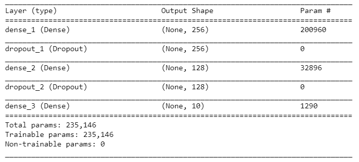
summary(model)

Here's the model's summary:

5. Next, we go ahead and compile our model by providing some appropriate arguments, such as theloss function, optimizer, and metrics. Here, we have used the rmsprop optimizer. This optimizer is similar to the gradient descent optimizer, except that it can increase our learning rate so that our algorithm can take larger steps in the horizontal direction, thus converging faster:

model %>% compile(
loss = 'categorical_crossentropy',
optimizer = optimizer_rmsprop(),
metrics = c('accuracy')
)

6. Now, let's fit the training data to the configured model. Here, we've set the number of epochs to 30, the batch size to 128, and the validation percentage to 20:

history <- model %>% fit(
                  x_train, y_train,
                  epochs = 30, batch_size = 128,
                  validation_split = 0.2
)

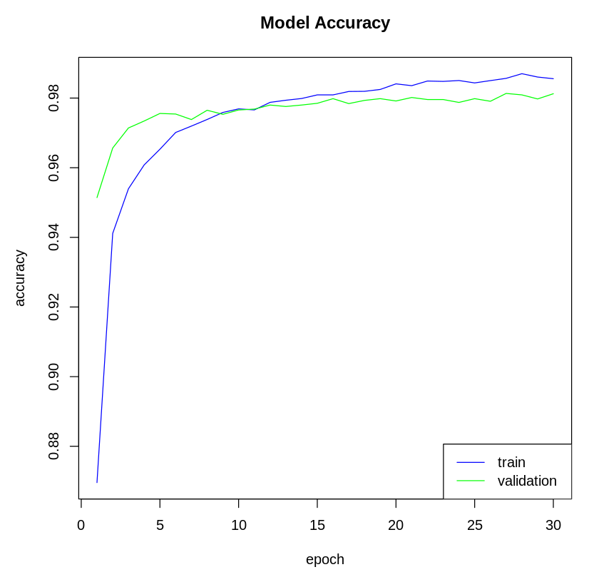
7. Next, we visualize the model metrics. We can plot the model's accuracy and loss metrics from the history variable. Let's plot the model's accuracy:

                  # Plot the accuracy of the training data
                  plot(history$metrics$acc,                  main=                  "Model Accuracy"                  ,                  xlab                  =                  "epoch"                  ,                  ylab=                  "accuracy"                  ,                  col=                  "blue"                  ,
                  type=                  "l"                  )                  # Plot the accuracy of the validation data
                  lines(history$metrics$val_acc,                  col=                  "green"                  )                  # Add Legend
legend(                  "bottomright"                  ,                  c                  (                  "train"                  ,                  "validation"                  ),                  col=                  c                  (                  "blue"                  ,                  "green"                  ),                  lty=                  c                  (                  1                  ,                  1                  ))                

The following plot shows the model's accuracy on the training and test dataset:

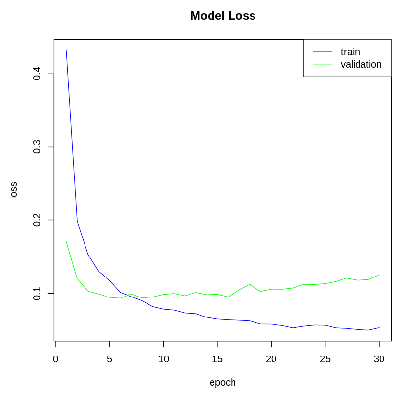
Now, let's plot the model's loss:

                  # Plot the model loss of the training data
                  plot(history$metrics$loss,                  main=                  "Model Loss"                  ,                  xlab                  =                  "epoch"                  ,                  ylab=                  "loss"                  ,                  col=                  "blue"                  ,                  type=                  "l"                  )                  # Plot the model loss of the validation data
                  lines(history$metrics$val_loss,                  col=                  "green"                  )                  # Add legend
                  legend(                  "topright"                  ,                  c                  (                  "train"                  ,                  "validation"                  ),                  col=                  c                  (                  "blue"                  ,                  "green"                  ),                  lty=                  c                  (                  1                  ,                  1                  ))                

The following plot shows the model's loss on the training and test dataset:

8. Now, we predict the classes for the test data instances using the trained model:

model                  %>%                  predict_classes(x_test)                

9. Let's check the accuracy of the model on the test data:

model %>% evaluate(x_test, y_test)

The following diagram shows the model metrics on the test data:

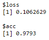
Here, we got an accuracy of around 97.9 %.

In step 1, w e loaded the MNIST dataset. The x data was a 3D array of grayscale values of the form (images, width, height). In step 2, we flattened these 28x28 images into a vector of length 784. Then, we normalized the grayscale values between 0 and 1. In step 3, we one-hot encoded the target variable using theto_categorical() function from keras to convert this into a binary format matrix.

In step 4, we built a sequential model by stacking dense and dropout layers. In a dense layer, every neuron receives input from all the neurons of the previous layer, which is why it's known as being densely connected.In our model, each layer took  input from the previous layer and applied an activation to the output of our previous layer. W e used therelu activation function in the hidden layers and the softmax activation function in the last layer since we had 10 possible outcomes. Dropout layers are used for regularizing deep learning models. Dropout  refers to the process of not considering certain neurons in the training phase during a particular forward or backward pass in order to prevent overfitting. The summary() function provides us with a summary of the model; it gives us information about each layer, such as the shape of the output and the parameters in each layer.

In step 5, we compiled the model using the compile() function from keras. We applied thermsprop() optimizer to find the weights and biases that minimize our objective loss function,categorical_crossentropy. The metrics argument calculates the metric to be evaluated by the model during training.

In step 6, we trained our model for a fixed number of iterations, which is defined by theepochs argument. The validation_split argument can take float values between 0 and 1 and specifies the fraction of the data to be used as validation data. Finally,batch_size defines the number of samples that will be propagated through the network. The history object records the training metrics for each epoch and contains two lists, params and metrics. The params contains the model's parameters, such as batch size, steps, and so on, while metrics contains model metrics such as loss and accuracy.

In step 7, we visualized the model's accuracy and loss metrics. In step 8, we used our model to generate predictions for the test data using thepredict_classes() function. Lastly, we evaluated the model's accuracy on the test data using the evaluate() function.

Tuning is the process of maximizing a model's performance without overfitting or underfitting. This can be achieved by setting appropriate values for the model parameters. A deep neural network has multiple parameters that can be tuned; layers, hidden units optimization parameters such as an optimizer, the learning rate, and the number of epochs.

To tune Keras model parameters, we need to define flags for the parameters that we want to optimize. These are defined by theflags() function of thekeras package, which returns an object of thetfruns_flags type. This contains information about the parameters to be tuned. In the following code block, we have declared four flags that will tune the dropout rate and the number of neurons in the first and second layers of the model. flag_integer("dense_units1",8) tunes the number of units in layer 1, dense_units1 is the name of the flag, and 8 is the default number of neurons:

# Defining flags
FLAGS <- flags(
                  flag_integer("dense_units1",8),
                  flag_numeric("dropout1",0.4),
                  flag_integer("dense_units2",8),
                  flag_numeric("dropout2", 0.3)
)

 Once we have defined the flags, we use them in the definition of our model. In the following code block, we have defined our model using the parameters that we want to tune:

# Defining model
model <- keras_model_sequential()
model %>%
                  layer_dense(units = FLAGS$dense_units1, activation = 'relu', input_shape = c(784)) %>%
                  layer_dropout(rate = FLAGS$dropout1) %>%
                  layer_dense(units = FLAGS$dense_units2, activation = 'relu') %>%
                  layer_dropout(rate = FLAGS$dropout2) %>%
                  layer_dense(units = 10, activation = 'softmax')

The preceding two code blocks are code snippets from the hyperparamexcter_tuning_model.R script, which is available in this book's GitHub repository. In the script, we have implemented a model for classifying MNIST digits. Executing this script does not tune your hyperparameters; it just defines the parameterized training runs to create the best model.

The following code block shows how we can fine-tune the model defined inhyperparameter_tuning_model.R . Here, we used thetuning_run() function from thetfruns  package. The tfruns package provides a suite of tools for tracking, visualizing, and managing TensorFlow training runs and experiments from R. The file argument of the function should be the path to the training script and should contain flags and the model definition. Theflags argument takes a list of key-value pairs where the key names must match the names of the different flags that we defined in our model. The tuning_run() function executes training runs for every combination of the specified flags. By default, all the runs go into the runs subdirectory of the current working directory. It returns a dataframe that contains summary information about all the runs, such as evaluation, validation and performance loss (categorical_crossentropy), and metrics (accuracy):

library(tfruns)
# training runs                    
runs <- tuning_run(file = "hypereparameter_tuning_model.R", flags = list(
                    dense_units1 = c(8,16),
                    dropout1 = c(0.2, 0.3, 0.4),
                    dense_units2 = c(8,16),
                    dropout2 = c(0.2, 0.3, 0.4)
))
runs
                

Here are the results from each run during hyperparameter tuning:

For each training run, we get the model metrics for the training and validation data.

• Vectorization of operations in deep neural networks:http://ufldl.stanford.edu/wiki/index.php/Neural_Network_Vectorization and https://peterroelants.github.io/posts/neural-network-implementation-part04/

Posted by: jacqueklann.blogspot.com

Source: https://www.packtpub.com/product/deep-learning-with-r-cookbook/9781789805673